From PPO to GRPO to DAPO: Understanding RL for LLMs and Every Training Parameter Explained

In our last post, we walked through how to fine-tune your own LLM using GRPO, Common Crawl, and Unsloth. We covered the full pipeline from data to deployment, but we intentionally skipped over something important: what do all those training parameters actually mean?

If you looked at the GRPOConfig block and thought "I just copied this and it worked, but I have no idea what half of these knobs do" — this post is for you. We're going to start from the beginning: what is PPO, how did GRPO improve on it, and what are the latest improvements like DAPO. Then we'll go parameter by parameter through the training config and explain what each one controls, in plain language, with analogies where they help.

The Big Picture: Teaching an AI to Get Better

Before we get into the alphabet soup of PPO, GRPO, and DAPO, let's set the stage with a simple analogy.

Imagine you're training a new chef. You've already taught them the basics — how to hold a knife, what ingredients go together, how recipes work. That's the pre-training phase of an LLM. The chef can cook, but their dishes aren't great yet.

Now you want to make them better. One approach: have them cook dishes, then give them feedback. "This was good, do more of that. This was bad, do less of that." That's reinforcement learning (RL). The chef tries things, gets scores, and adjusts. PPO, GRPO, and DAPO are all different strategies for how you deliver that feedback and how aggressively the chef should change their cooking based on it.

PPO: The Original Heavyweight

PPO (Proximal Policy Optimization) was the go-to method for RLHF (Reinforcement Learning from Human Feedback) in early ChatGPT-style models. It works, but it's expensive. To understand why, let's go back to our chef analogy.

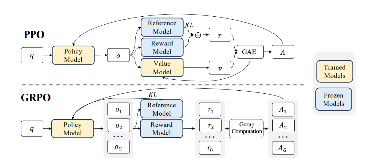
PPO is like running a kitchen with four people involved at all times. First, there's the chef you're training (the policy model). Second, there's a copy of the chef from last week, frozen in time, who you compare against to make sure the current chef doesn't change too drastically (the reference model). Third, there's a food critic who scores every dish (the reward model). And fourth, there's an assistant who tries to predict how good a dish will be before it's even finished — a "gut feeling" estimator (the value model). All four of these need to be loaded in GPU memory at the same time. For a 7B parameter model, that means you need enough memory for roughly four copies of the model. That's why PPO requires serious hardware — often multiple high-end GPUs just to get started.

The value model is especially tricky. Its job is to estimate "how much reward will this sequence of tokens eventually get?" at every single token position. Training this value model well is itself a hard problem, and if it's wrong, it gives the chef bad advice.

GRPO: The Lean Alternative

GRPO (Group Relative Policy Optimization) was introduced by DeepSeek in their DeepSeekMath paper. The key insight was: do we really need that value model? What if, instead of predicting how good a dish will be, we just make the chef cook multiple dishes and compare them against each other?

Here's how GRPO works. Give the model a prompt — say, a math problem. Instead of generating one answer, generate a group of answers (say 4, 8, or 16). Score each answer with a simple reward function: did it get the right number? Did it follow the format? Then normalize the scores within the group by subtracting the mean and dividing by the standard deviation. The answers that scored above average get reinforced (the model learns to do more of that), and the ones below average get penalized (the model learns to avoid that).

Think of it like a cooking competition. Instead of one expert critic telling the chef what's good (PPO's value model), the chef cooks 8 versions of the same dish, a simple scoring checklist rates them, and the chef learns by comparing the good ones against the bad ones in that batch. That's the "Group Relative" part — the evaluation is always relative within the group.

This has two massive advantages over PPO. First, no value model means you cut your memory usage significantly — you only need the training model and optionally a reference model, not four models. Second, no trained reward model is needed. Instead of training a separate neural network to judge quality (which itself requires expensive human-labeled preference data), you write simple Python functions: "Is the answer correct? Is the format right?" This is sometimes called RLVR — Reinforcement Learning with Verifiable Rewards.

The practical result: GRPO makes reinforcement learning for LLMs feasible on a single GPU. That's why we used it in our last post, and it's why DeepSeek used it to train their R1 reasoning models.

DAPO: Fixing GRPO's Rough Edges

GRPO was a big leap forward, but as people scaled it up, they found some issues. DAPO (Decoupled Clip and Dynamic Sampling Policy Optimization) was introduced in early 2025 to address these problems. Think of DAPO as "GRPO with the lessons learned from running it at scale." There are several key improvements.

Length bias fix. Original GRPO normalizes its loss by dividing per sequence length. This sounds reasonable, but it creates a sneaky problem: shorter answers with positive rewards get disproportionately large gradient updates, while longer answers get diluted. Imagine two chefs in a competition — one writes a one-line answer, the other writes a full essay. If both are equally correct, the one-liner gets more credit per word. DAPO fixes this by normalizing across all tokens in the batch rather than per sequence, treating every token's contribution more fairly.

Decoupled clipping. In standard GRPO (borrowed from PPO), there's a single clip range that limits how much the model can change in one step. DAPO decouples this into separate upper and lower bounds. Why? Because when the model produces a bad answer and tries to move away from it, you want to let it move further. But when it produces a good answer and tries to lean into it too hard, you want tighter control to prevent instability. In TRL's implementation, you can set different values for epsilon (lower bound) and epsilon_high (upper bound) to get this behavior.

No KL penalty. GRPO originally included a KL divergence term to keep the model from drifting too far from its starting point. But multiple research groups found that for reasoning tasks with verifiable rewards, this penalty isn't necessary and can actually hurt performance by being too conservative. DAPO drops it entirely (beta = 0), and TRL now defaults to this as well.

Truncation masking. If the model generates a response that hits the maximum length limit and gets cut off, it's an incomplete thought. Training on truncated responses introduces noise — the model gets penalized for something it didn't finish. DAPO masks these truncated completions from the loss calculation entirely. You can enable this with mask_truncated_completions=True in TRL.

A Quick Summary: PPO vs GRPO vs DAPO

PPO requires four models in memory (policy, reference, value, reward), uses a trained reward model, and is computationally expensive. It's the proven workhorse but needs serious hardware.

GRPO removes the value model, replaces the trained reward model with simple Python functions, and uses group-based comparison instead. Dramatically less memory, runs on a single GPU.

DAPO takes GRPO and fixes length bias in the loss function, adds asymmetric clipping for better stability, drops the KL penalty, and masks truncated completions. It's now the default loss type in TRL's GRPOTrainer.

Now Let's Talk About Every Parameter

Here's the GRPOConfig from our last post. Let's go through every single parameter and explain what it does.

training_args = GRPOConfig(
    learning_rate = 5e-6,
    adam_beta1 = 0.9,
    adam_beta2 = 0.99,
    weight_decay = 0.1,
    warmup_ratio = 0.1,
    lr_scheduler_type = "cosine",
    optim = "adamw_torch_fused",
    logging_steps = 1,
    per_device_train_batch_size = 1,
    gradient_accumulation_steps = 1,
    num_generations = 4,
    max_prompt_length = 256,
    max_completion_length = max_seq_length - 256,
    max_steps = 50,
    save_steps = 50,
    max_grad_norm = 0.1,
    report_to = "none",
    output_dir = "outputs",
)

learning_rate = 5e-6

The learning rate controls how big of a step the model takes when updating its weights after each batch. Think of it like the size of a stride when hiking down a mountain toward the lowest valley. Too large, and you overshoot and stumble past the good spot. Too small, and you barely move and training takes forever.

For GRPO fine-tuning, 5e-6 (that's 0.000005) is quite conservative — and that's usually what you want. You're starting from a model that already knows a lot, and you want to nudge it gently, not overhaul its entire personality. If training seems too slow, you might bump it up to 1e-5. If the model starts outputting garbage mid-training, try making it even smaller.

adam_beta1 = 0.9 and adam_beta2 = 0.99

These control the Adam optimizer's "momentum." Adam doesn't just look at the current gradient — it remembers past gradients and uses that memory to smooth out its updates.

adam_beta1 (0.9) controls how much the optimizer remembers about the direction of recent gradients. Think of it like a ball rolling down a hill — beta1 determines how much inertia the ball has. At 0.9, the optimizer heavily considers the last ~10 steps of direction, which helps it push through noisy updates without zigzagging. A value of 0.0 would mean "no memory, react only to the current gradient."

adam_beta2 (0.99) controls how the optimizer tracks the magnitude of recent gradients. This helps it adapt the learning rate for each individual parameter. Some parameters need big updates, others need small ones. Beta2 at 0.99 means it averages over roughly the last 100 steps to estimate this. The value 0.99 (instead of the more common 0.999) is a DeepSeek recommendation for GRPO — it makes the optimizer slightly more responsive to recent changes in gradient magnitude, which helps with the noisier reward signals you get in RL training.

weight_decay = 0.1

Weight decay is a regularization technique that gently pushes the model's weights toward zero over time. Imagine every parameter in the model has a slight pull back toward its "default" — it prevents any single weight from growing absurdly large and dominating the model's behavior.

At 0.1, this is a moderate amount of regularization. It helps prevent overfitting, especially when your training dataset is small. Think of it as gravity — it keeps the model grounded and prevents it from memorizing the training data rather than learning general patterns. If you were training on a very large dataset, you might lower this; with a small dataset, you might even increase it slightly.

warmup_ratio = 0.1

Training doesn't start at full speed. The warmup ratio says "for the first 10% of training steps, gradually ramp up the learning rate from near zero to the target value."

Why? Imagine you're a musician who hasn't played in a while. You don't start a concert with the hardest piece at full tempo — you warm up with scales first. Similarly, at the start of training, the model's gradients can be wild and unpredictable, especially in RL where the reward signal is noisy. Starting with tiny updates lets the optimizer calibrate before it starts taking big steps. With max_steps = 50 and warmup_ratio = 0.1, the first 5 steps will be warmup.

lr_scheduler_type = "cosine"

After warmup, the learning rate doesn't stay constant — it follows a schedule. "Cosine" means the learning rate decreases following the shape of a cosine curve: it stays near the peak for a while, then gradually slows down toward the end of training.

Think of it like running a race. You start at a good pace (after warmup), maintain it through the middle, and then ease into the finish. The idea is that early in training you want bigger updates to make progress, but as you get closer to a good solution, you want smaller, more precise adjustments. The cosine shape is popular because it provides a smooth, gradual decay rather than an abrupt drop.

optim = "adamw_torch_fused"

This selects which optimizer implementation to use. AdamW is the standard optimizer for training modern neural networks — it's Adam with a corrected weight decay implementation. The "torch_fused" part means it uses PyTorch's fused CUDA kernel, which runs the optimizer math directly on the GPU in a single operation instead of multiple separate operations.

In practice, "adamw_torch_fused" is about 5-10% faster than the non-fused version. There's no quality difference — it computes the exact same math, just more efficiently. Always use this if you're training on a CUDA GPU.

logging_steps = 1

This controls how often training metrics (loss, reward, learning rate, etc.) are printed or logged. Setting it to 1 means "log every single step." With only 50 total steps in our training run, you definitely want to see what's happening at every step. If you were running for 10,000 steps, you'd probably set this to 10 or 50 to avoid flooding your terminal.

per_device_train_batch_size = 1

This is how many prompts are processed per GPU in each training step. With a batch size of 1, each step processes exactly one prompt. Combined with num_generations = 4, that means each step generates 4 completions for that 1 prompt, scores them, and updates the model.

We're using 1 here because of memory constraints on a free Colab T4 (16GB VRAM). Each prompt generates multiple completions, and all of those need to fit in memory. Larger batch sizes give more stable gradient estimates but require more VRAM. If you have an A100 (80GB), you could bump this to 4 or 8.

gradient_accumulation_steps = 1

This is a trick for simulating a larger batch size without needing the memory for it. If you set this to 4, the model would process 4 separate batches, accumulate their gradients, and then do one big update. The effect is the same as having a batch size 4x larger.

Think of it like taking notes during a meeting. Instead of acting on every single note immediately (steps=1), you could accumulate notes for 4 topics and then take action on all of them at once (steps=4). The end result is the same, but you make one bigger, more informed decision instead of many small reactive ones. We set it to 1 here because our batch size is already minimal.

num_generations = 4

This is the most important GRPO-specific parameter. It controls how many completions the model generates for each prompt in the group comparison. Remember the core idea of GRPO: generate multiple answers, score them, reinforce the good ones and penalize the bad ones.

With num_generations = 4, the model generates 4 different answers for each math problem. The reward functions score all 4, and the model learns from the contrast between the best and worst responses. More generations means better gradient estimates — it's like asking 4 vs 16 people for opinions. More opinions give you a better sense of the consensus.

4 is the minimum we'd recommend. If you have more VRAM, try 8 or 16. The DeepSeek team used values as high as 64 for their production training runs. But each generation costs memory and compute, so this is often the bottleneck on consumer hardware.

max_prompt_length = 256

The maximum number of tokens allowed for the input prompt. Any prompt longer than this gets truncated. This saves memory by ensuring the model doesn't have to process extremely long inputs.

For GSM8K math problems, 256 tokens is plenty — most problems are only a few sentences. If you're working with longer inputs (code, legal documents, medical notes), you'd need to increase this. Just remember that every token costs memory, and the total (prompt + completion) is what really matters.

max_completion_length = max_seq_length - 256

The maximum number of tokens the model can generate as a response. In our setup, max_seq_length is 1024, so this works out to 768 tokens. The model's working memory is divided between reading the prompt and writing the response — this parameter sets the boundary.

If the model hits this limit, it stops generating mid-thought. That's usually undesirable (the response is incomplete), which is why DAPO introduced truncation masking. You want this long enough for the model to finish its reasoning, but not so long that you waste VRAM on empty token slots.

max_steps = 50

The total number of training steps to run. Each step processes one batch, generates completions, scores them, and updates the model weights. 50 steps is a very short training run — essentially a quick proof of concept.

For real fine-tuning, you'd typically want hundreds to thousands of steps depending on your dataset size and task complexity. But 50 steps is enough to see whether the reward is trending upward and confirm your setup is working. Think of it as a test drive — you don't need to drive 1,000 miles to know if the car runs.

save_steps = 50

Save a checkpoint every N steps. With save_steps = 50 and max_steps = 50, we only save at the end of training. For longer runs, you'd want to save more frequently (e.g., every 100 or 200 steps) so you can resume training if something crashes, or go back to an earlier checkpoint if the model starts degrading.

max_grad_norm = 0.1

Gradient clipping. If the gradient (the "direction and magnitude" of the weight update) gets too large, this clips it down to a maximum norm of 0.1. This is like putting a speed limit on your weight updates.

Why would gradients get too large? In RL training, reward signals can be noisy and cause occasional "gradient explosions" — one bad batch can produce an enormous gradient that sends your model off a cliff. Clipping at 0.1 is quite aggressive (the default in TRL is 1.0), meaning we're being very conservative about update sizes. For GRPO with small models and limited steps, this is a good safety net. If you're seeing training instability, try lowering this further. If training is too slow to converge, try raising it to 0.5 or 1.0.

report_to = "none"

This controls where training metrics are sent. "none" means no external reporting — metrics only show in the console. Other options include "wandb" (Weights & Biases), "tensorboard", or "mlflow" for experiment tracking. For a quick Colab experiment, "none" keeps things simple. For production training runs, you'd want to use one of the tracking services to monitor training curves across experiments.

output_dir = "outputs"

Where checkpoints and logs are saved on disk. Straightforward — the model weights will be saved to the "outputs" folder. In Colab, remember this is ephemeral storage unless you mount Google Drive.

The Reward Functions: Where the Magic Happens

Beyond the config parameters, the other critical piece is the reward functions you pass to GRPOTrainer. These are just plain Python functions that score completions — no neural network required.

trainer = GRPOTrainer(
    model = model,
    processing_class = tokenizer,
    reward_funcs = [
        match_format_exactly,
        match_format_approximately,
        check_answer,
        check_numbers,
    ],
    args = training_args,
    train_dataset = dataset,
)

Each reward function receives the prompts and completions, and returns a list of float scores. The scores from all functions are summed for each completion. In our setup, match_format_exactly gives 3 points for perfect format compliance, match_format_approximately gives partial credit, check_answer gives 3 points for a correct answer (or -1 for a wrong one), and check_numbers gives small rewards for having the right numbers in the response.

The beauty of this approach is that you can stack rewards and weight them however you want. You can add new reward functions without changing anything else. Want to penalize responses that are too long? Add a length penalty function. Want to reward proper citations? Add a citation checker. The reward function design is where you should spend most of your iteration time — it's the clearest lever you have for shaping model behavior.

Parameters We Didn't Use (But You Should Know About)

Our config was fairly minimal. Here are a few important GRPOConfig parameters we left at their defaults that you might want to tune for production runs.

beta (default: 0.0) — The KL divergence penalty coefficient. At 0.0, there's no penalty for the model drifting from its starting weights. If you're worried about the model "forgetting" its pre-training knowledge, set this to a small value like 0.001 (what DeepSeek R1 used). This adds a cost for being too different from the original model, acting like a rubber band pulling the model back.

num_iterations (default: 1) — How many gradient updates to perform per batch of generations. At 1, each group of generations is used for exactly one weight update. Higher values reuse the same batch for multiple updates (like PPO's "epochs per batch"), which can be more sample-efficient but risks overfitting to that batch.

epsilon (default: 0.2) — The clip range for the policy ratio. This prevents any single update from changing the model too dramatically. At 0.2, the ratio between old and new policy probabilities is bounded to [0.8, 1.2]. Larger values allow bigger per-step changes; smaller values are more conservative. DAPO recommends using different upper and lower bounds via epsilon_high.

temperature (default: 1.0) — Controls randomness during generation. At 1.0, the model samples normally. Higher values (1.5, 2.0) make it more creative and diverse. Lower values (0.5) make it more deterministic. For GRPO, you generally want some diversity in generations so the model has a range of good and bad examples to compare — so 1.0 or slightly higher is usually good.

loss_type (default: "dapo") — Which loss formulation to use. As discussed earlier, "dapo" is the newest and fixes length bias. Other options include "grpo" (the original, has length bias), "dr_grpo" (fixes length bias by dividing by max completion length), and "sapo" (uses soft gating instead of hard clipping).

scale_rewards (default: "group") — How to normalize rewards. "group" divides by the standard deviation within each group. "batch" divides by the batch-wide standard deviation. False disables normalization entirely. The Dr. GRPO paper argues that group-level std normalization introduces difficulty bias (easy questions get inflated gradients because all answers are similar), so you might want to try False or "batch" for production runs.

Putting It All Together

If you zoom out, the parameter choices in our config follow a clear philosophy: be conservative, stay within memory limits, and prioritize stability over speed.

The learning rate is small (5e-6), gradient clipping is tight (0.1), weight decay provides regularization (0.1), warmup eases into training (10% of steps), cosine scheduling smoothly reduces the learning rate, batch size is minimal (1) to fit in Colab's memory, and we run just enough steps (50) to see if it's working.

For a production run, you'd likely increase the batch size, run for more steps, use a larger num_generations, and set up proper experiment tracking. But the fundamentals don't change — these same parameters control the same trade-offs whether you're on a T4 or an H100 cluster.

The most impactful things to tune, in order: your reward functions (by far the most important), num_generations, learning_rate, max_steps, and then everything else. Get the rewards right first, then tune the training dynamics.

Like, Share, and Subscribe ^ _ ^

If you have questions about any of these parameters or want help adapting this setup for your own use case, drop us a line. And if you're looking for help going from prototype to production with fine-tuned models — that's what we do at SoftmaxData.