Lately, we have been customizing LSTM layer for a Natural Language Generation project. As a result, I have been going through Keras’ LSTM source code and want to share some of my understanding. Hopefully my limited knowledge would benefit you in some shape or form.
Alright, let’s jump right in.
Where to find the source code
Keras’ source code is publicly available here.
It seems that the team put all recurrent layers in a single file. There are a few things you need to understand before you decide to move on here:
- What is LSTM and the detailed computation?
- How a Keras layer works?
Let’s briefly touch the two items.
LSTM and the computation behind it
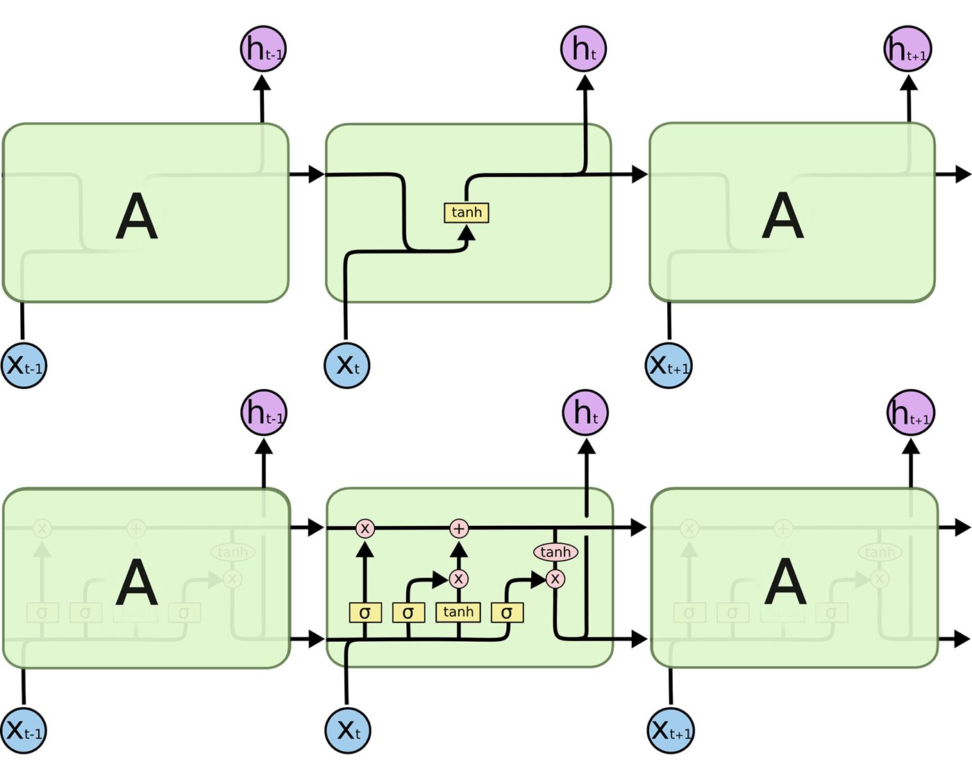
Chris Olah had a great blog explaining LSTM . I highly recommend reading it if you cannot visualize the cells and the unrolling process.
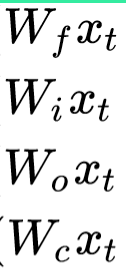
There is one caveat: the notation he used is not directly corresponding to the source code. For example:
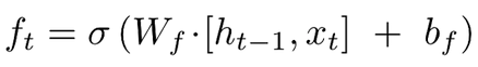
Which denotes a forget gate weight Wf. However, this did not sufficiently address the detailed computation that’s happening inside Kera’s source code. I actually found the equations listed on Wikipedia’s LSTM page is a much better visualization of the detailed computation.
For the rest of this writing, I will exclusively use Wikipedia’s equations.
Ok, let’s move on.
The idea behind LSTM cells is that the network is able to remember as well as forget information of the previous timestep.
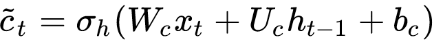
So, first, you have a “Forget Gate” that’s responsible for determining whether previous information should pass through:

Xt here is the current input while ht-1 is the previous timesteps’ output after passing through an output gate. If you are not sure what this means, you need to go back, read the paper or Chris’s blog or other literature on the topic.
There are effectively three individual weights here:
- Wf: input weight for the forget gate
- Uf: recurrent weight for the forget gate
- bf: bias weight for the forget gate
Wf denotes the weight of the forget gate for the current timestep’s input while Uf denotes the recurrent weight of the forget gate for the previous timestep’s cell state. bf is simply a bias weight.
You will notice it uses a Sigmoid function, which means it produces an output between 1 and 0. So it can determine which parts of the previous cell state are to be forgotten or kept. Sigmoid function is used quite a few times throughout the LSTM cell computation because of the “gate” nature, where information is passed through or filtered out. In Keras’ actual implementation, you are allowed to choose this activation function with a variable named “recurrent_activation” .
Next, we need to figure out whether we should update parts of the cell with current input. This gate is called update gate:

Again, you can see it uses Sigmoid function to determine whether to let pieces of information pass through. Now you see another three weights to be trained:
- Wi: input weight for the update gate
- Ui: recurrent weight for the update gate
- bi: bias weight for the update gate.
Now, we cannot just input a raw value and let it do a dot multiplication with the update gate. Just like any other cell operation, it needs to have weights that governs how much information passes through.
So we need a candidate value that derived from the current input. In a lot of literature, they are called update candidate value.
Just like all other tensor operations, this candidate value requires three sets of weight:
- Wc: input weight for the candidate value
- Uc: recurrent weight for the candidate value
- bi: bias weight for the candidate value
With the gates ready and candidate values ready, we now need to combine them together to form the final candidate value:
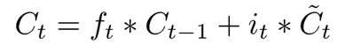
What this equation means is that, first it will determine whether parts of the cell state of the previous timestep should be taken into account with a “forget gate”; next, it will use an update gate to determine whether current input should be combined with the previous timestep to form the output candidate value of the current timestep. This is nothing uncommon among RNN networks where it leverages the “memory” of other steps to affect the output.
Now that we have a candidate value, we need to produce the output cell state of the current timestep. Just like any other steps, we need a gate to govern which pieces of the cell state to be produced.

Here, we see another set of three weights:
- Wo: input weight for the output gate
- Uo: recurrent weight for the output gate
- bo: bias weight for the output gate
Next, we combine the candidate value with the output gate to produce the final output:
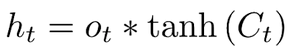
At this step, the ht can be passed to the next timestep along with the raw candidate value Ct.
There is one thing to keep a note of: this equation used Tanh activation on the candidate value, Keras’ implementation actually allows you to use a different type of activation function such as ReLU.
Now, let’s pause for a second, and count the number of weights we have seen:
- Wf: input weight for the forget gate
- Uf: recurrent weight for the forget gate
- bf: bias weight for the forget gate
- Wi: input weight for the update gate
- Ui: recurrent weight for the update gate
- bi: bias weight for the update gate.
- Wc: input weight for the candidate value
- Uc: recurrent weight for the candidate value
- bi: bias weight for the candidate value
- Wo: input weight for the output gate
- Uo: recurrent weight for the output gate
- bo: bias weight for the output gate
So there you have it, there are 12 weights that can largely be divided into three camps:
- input weight that multiplies with the input timestep
- recurrent weight that multiplies with the previous output
- bias weight
Each camp contains four sets of weights.
The weights and bias of each camp have the same dimension and can be stacked together. The list of weights and biases above is crucial for later understanding of the source code.
Now, let’s talk about Keras layer in general.
How Keras layer works
Before we jump into RNN specifics, I recommend you take a look at Kera’s documentation. In short, a layer class requires a few core functions:
- build(), which is called to define weights.
- call() , this is the main part of a layer class. It’s called to perform the computation.
- compute_output_shape(), this is pretty self-explanatory what it does.
So what you need to keep an eye on when reading the source code are build() and call().
Understanding Keras LSTM layer
Keras LSTM layer essentially inherited from the RNN layer class. You can see in the __init__ function, it created a LSTMCell and called its parent class.
Let’s pause for a second and think through the logic. LSTM is a type of RNN. The biggest difference is between LSTM and GRU and SimpleRNN is how LSTM update cell states. The unrolling process is exactly the same. Therefore, it makes sense that Keras LSTM defines its own cell and then use RNN’s general unrolling process.
Let’s summarize it a little:
- A Cell in RNN governs how one particular timestep is updating the state. This is where the actual computation happens.
- A RNN layer wraps around Cell and unroll multiple timesteps to update the cell date.
Think of RNN as a big for loops that update the Cell throughout the timesteps.
There are a lot of functions and properties inside an RNN class. However, our focus here is the LSTMCell and how it does the computation.
Understanding LSTMCell
Recall that there are two functions we need to pay attention to:
- build(), which sets the weight
- call(), which does the computation between weights and input.
Understanding LSTMCell’s build() function
First, let’s go into details of build() and see how it is defining its own weights:
The most important lines here are:
- Line 12: initializing the input weight tensor
- Line 17: initializing the recurrent weight tensor
- Line 35: initializing the bias weight tensor
- Line 45–65: slicing the weights of each camp into individual weight.
Let’s go through these lines
The cell effectively has three traininable weight tensors. They are called kernel and recurrent_kernel respectively. They are corresponding to the three camps of weights we talked about earlier.
Let’s take a look at Line 12 first.
self.kernel = self.add_weight(shape=(input_dim, self.units * 4), name=’kernel’, initializer=self.kernel_initializer, regularizer=self.kernel_regularizer, constraint=self.kernel_constraint)
It defines the input weight. What you need to pay attention to here is the shape.
The input_dim is defined as
input_dim = input_shape[-1]
Let’s say, you have a sequence of text with embedding size of 20 and the sequence is about 5 words long. So the input_shape = (5, 20).
input_shape[-1] = 20.
Obviously, a length of 5 is more important to RNN layer when unrolling. So the cell itself is only interested in a single input at one timestep. That’s why it uses the last of the shape tuple.
self.units is the number of neurons of the LSTM layer. Say you want 32 neurons, then self.units=32. But, why it needs 4 times of the neurons as the second dimension rather than just the number of neurons? Recall early we have the 12 weights divided into three camps? Each camp contains 4 weights.
It essentially is stacking all the weights of the input weight camp together and then later uses slicing to individually update this giant weight tensor.
In fact, you can see between line 43 and line 46.
self.kernel_i = self.kernel[:, :self.units]
self.kernel_f = self.kernel[:, self.units: self.units * 2]
self.kernel_c = self.kernel[:, self.units * 2: self.units * 3]
self.kernel_o = self.kernel[:, self.units * 3:]
Let’s uses the simpliest example: you only have 1 neuron in this layer. Your input is a 5 element long sequence and each element of the sequence is 20 dimension. For example, think of processing 5 words each time and each word is embedded into 20 dimensions.
self.kernel would have a shape of (20, 4): 20 rows and 4 columns. Each column is one input weight.
They stand for Wi, Wf, Wc and Wo in our earlier notations respectively.
Let’s stop here for a second. Each input at each timestep has a shape of (1, 20) (each word is embedded into 20 dimensions).
That’s why each input weight’s shape should start with the same dimension 20 when computing the tensors.
The same technique has been used on the recurrent weight camp (U weight in our notation).
Line 17 is where they initialized the recurrent weight:
self.recurrent_kernel = self.add_weight( shape=(self.units, self.units * 4), name=’recurrent_kernel’, initializer=self.recurrent_initializer, regularizer=self.recurrent_regularizer, constraint=self.recurrent_constraint)
Then they are sliced into individual recurrent weight:
self.recurrent_kernel_i = self.recurrent_kernel[:, :self.units]
self.recurrent_kernel_f = ( self.recurrent_kernel[:, self.units: self.units * 2])
self.recurrent_kernel_c = ( self.recurrent_kernel[:, self.units * 2: self.units * 3])
self.recurrent_kernel_o = self.recurrent_kernel[:, self.units * 3:]
They represent Ui, Uf, Uc, Uo weights in our notations.
Now you may ask, why would the shape be different from the input weight? That’s because they are multiplying by different types of variables.
kernel weight (input weight) multiply by an input tensor , while recurrent kernel multiplies by the previous timestep’s output tensor ht-1.
Let’s go back to the example earlier, where the input sequence has a shape of (5,20). At each timestep, the cell has an input of (1,20). Assuming, we have 32 neurons. At timestep zero, there is no previous timestep, so ht-1 can be omitted.
Then the output of the tensor should be (1,20) dot (20, 32). The output becomes (1,32)
The recurrent weight should have a shape of (number of neurons, number of neurons) so that it can maintain the output shape. In our example (32, 32)
Then (1,32) dot (32, 32) becomes (1,32), that’s how you can combine the weights together with input weight dot input.
The shape is very crucial when reading the code. Because it didn’t use individual weights; instead, it uses stacking so that the tensor computation is sped up by doing all the multiplication at once.
Finally, the same goes with bias weights, where it intializes 4 times of the number of units and stack the weights together (Line 35)
self.bias = self.add_weight(shape=(self.units * 4,), name=’bias’, initializer=bias_initializer, regularizer=self.bias_regularizer, constraint=self.bias_constraint)
Then slice them into different biases:
self.bias_i = self.bias[:self.units]
self.bias_f = self.bias[self.units: self.units * 2]
self.bias_c = self.bias[self.units * 2: self.units * 3]
self.bias_o = self.bias[self.units * 3:]
Of course, should you choose not to use bias, this step is omitted.
Pew, you survived the build() function. Let’s move on to the call function,
Understanding LSTMCell’s call() function
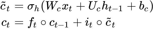
Before we move on, let me remind you of the computations:
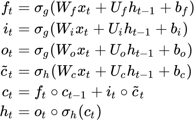
Let’s compare these equations line by line in Kera’s source code below:
Line 2–19 are effectively about dropout. It’s easy to understand as it is creating dropout masks and multiple the masks with weight tensors. Let’s not spend too much time on that unless you are into how dropout works.
At each timestep, two things are computed as output:
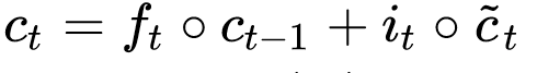
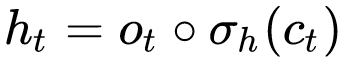
Ct means the carry state of the timestep (raw candidate value) while ht is the memory of the previous timestep (the final output after having the candidate value go through a Tanh activation and then dot an output gate).
They actually mean very different things. Ct means the cell state of the previous timestep. But we put that inside a Tanh function so that the value will be between (-1 and 1) then multiply it by an output gate, so that only parts of the output are kept. Think of Ct as the raw shareholder report while ht as the refined and filtered version of a report, which is the balance sheet + income statement.
When Ct and ht are given to the next timestep, they are denoted as Ct-1 and Ht-1 respectively. In the source code of Keras (line 21, 22) they used variable
h_tm1 and c_tm1 (I am guessing tm means time minus?)
At line 24, there is a if statement asking which implementation mode (1 or 2). According to the official documentation:
Implementation mode, either 1 or 2. Mode 1 will structure its operations as a larger number of smaller dot products and additions, whereas mode 2 will batch them into fewer, larger operations. These modes will have different performance profiles on different hardware and for different applications.
I personally find mode = 1 is the easiest to undertand given our equations, although the default is actually 2. Mode 2 has much fewer lines of code because it comebines a lot of the weight computation together. They are nevertheless the same. I’d encourage you to try them out individiually on your local setup to see which one works better with your hardware.
Line 31–34, effectively replicate the input timestep to four individual variables:
inputs_i = inputs
inputs_f = inputs
inputs_c = inputs
inputs_o = inputs
They also replciate the output of the previous timestep h_mt1 four times by the same token (line 51–54):
h_tm1_i = h_tm1
h_tm1_f = h_tm1
h_tm1_c = h_tm1
h_tm1_o = h_tm1
In mode 2, they didn’t do that. I have no idea under what hardware setup this would speed things up. Nevertheless, the input variable corresponds to Xt in our notations.
To compute each gate and candidate value, first we need to multiply the kernel weight by input:
In Keras’ code, it assigned differant variables that temporarily store these values called x_f, x_i, x_o, x_c respectively. You can actually see them between line 35–38.
x_i = K.dot(inputs_i, self.kernel_i)
x_f = K.dot(inputs_f, self.kernel_f)
x_c = K.dot(inputs_c, self.kernel_c)
x_o = K.dot(inputs_o, self.kernel_o)
Once that’s computed and if you want to use bias weights, they added the variable to bias weights and overwrite the variable values (line 40–43):
x_i = K.bias_add(x_i, self.bias_i)
x_f = K.bias_add(x_f, self.bias_f)
x_c = K.bias_add(x_c, self.bias_c)
x_o = K.bias_add(x_o, self.bias_o)
Now, let’s go back to the individual equations we had earlier:
This is corresponding to line 57–58:
f = self.recurrent_activation(x_f + K.dot(h_tm1_f, self.recurrent_kernel_f))
Please note that they used recurrent_activation to activate instead of the standard Sigmoid function. The reason is because you can actually change this function when intializing the cell. By default, it is Sigmoid.
This update gate computation is corresponding to line 55:
i = self.recurrent_activation(x_i + K.dot(h_tm1_i, self.recurrent_kernel_i))
The same as earlier, they used recurrent_activation instead of Sigmoid.
Output gate is corresponding to line 61:
o = self.recurrent_activation(x_o + K.dot(h_tm1_o, self.recurrent_kernel_o))
The candidate value is corresponding to line 59:
c = f * c_tm1 + i * self.activation(x_c + K.dot(h_tm1_c, self.recurrent_kernel_c))
Few things to note here:
- In our notation there activation function (Tanh by default) wasn’t clear.
- In Keras’ code, the author used self.activation. You can also use ReLU, by default it should be Tanh.
- The single line of code combined the two equations together, I think it’s a little harder to read than the other lines.
Now we have the candidate value, the output gate, we should compute the output of the current timestep
This is corresponding to line 83:
h = o * self.activation(c)
Again, it used self.activation instad of Tanh in the original paper. I found in practice, a lot of folks used ReLU instead.
Finally, it returns this output as well as the raw candidate value (line 87)
return h, [h, c]
Going back to LSTM Layer code
The LSTM Layer doesn’t implement any specific code inside Call(). Instead, it just calles it’s parent class (RNN layer) to execute the unrolling.
This is because in terms of unrolling itself, it has nothing particularly special.
Let’s take a look at how RNN’s call() does it.
Understandingly, the code contains a lot of checking. The meat of the logic starts at line 54, where it acquires the shape of the inputs.
Say, you have 1000 sequences, each sequence is 10 elements and each element is embedded in a 20 dimension space. So the input shape is (1000, 10, 20)
The timestep should be 10. That’s why you are seeing line 55:
timesteps = input_shape[1]
In the simplest way to imagine this process is that we are going to repeat the LSTMCell 10 times and each time, we will give the previous timestep’s cell state that it computed earlier.
This effectively is what line 86 is about:
last_output, outputs, states = K.rnn(step, inputs, initial_state, constants=constants, go_backwards=self.go_backwards, mask=mask, unroll=self.unroll, input_length=timesteps)
In Keras, you can demand the layer to return a Sequence instead of the last timestep’s output by turning return_sequences=True. This is required when you are stacking multiple LSTM together. Because LSTM requires an input of three dimension tensor.
This is what line 100–103 are about:
if self.return_sequences:
output = outputs
else:
output = last_output
I understand this is a very lengthy explanation. Hopefully, it helps you understanding LSTM as well as how Keras implemented it. Have questions? Leave a comment or email me: jia AT softmaxdata.com